Why a Continuous Joint Module Size Range Beats Point Optimization
Explore a continuous joint module size range (40mm-190mm). Overcome interface fragmentation and optimize robot joint selection with integrated actuators.
 September 28, 2026

 > Why a Continuous Joint Module Size Range Beats Point Optimization
 A joint module is an integrated actuator that combines a strain wave gears, a servo motor, an absolute encoder, and a servo drive in one housing. An arm designer therefore specifies one torque and position unit instead of a stack of separate parts. Its mechanical and electrical interfaces are defined by the selected configuration, helping simplify system integration and commissioning.
Comparing modules by data sheet value is normal practice, and sufficient for a single component. At machine level the same method omits the cost of joining modules from different engineering systems. This article treats the joint module size range as one continuous design space. It gives the engineering case for a complete 40 mm to 190 mm spectrum over a short list of individually strong parts.
Laifual Drive covers a continuous joint module outside-diameter range from 40 mm to 190 mm, spanning multiple low-voltage and high-voltage configurations. That range links to harmonic reducer sizes 3 through 58 and outer diameters of 13 mm to 246 mm. Later sections define the cost a discontinuous spectrum creates. They then give the parameter definitions, size data, protocol set, and selection procedure.
Technical Background: Interface Fragmentation and Its Engineering Cost
Module comparison usually happens at the parameter level, which is right for a part but not for a machine: four costs follow from mixing modules from different engineering systems.
Interface Fragmentation Across Suppliers
Interface fragmentation is the first. Flange dimensions, mounting hole patterns, and cable routing are defined by each supplier independently. A machine that mixes suppliers therefore needs adapter plates, custom harnesses, and reworked structural parts. Its real cost is not the adapter plate but the redesign loop it forces on the arm structure and the cable path inside it.
Specification Gaps in the Catalog Middle
Specification gaps are the second. Catalogs are often complete at both ends and empty in the middle. An axis in the gap then has two answers: accept a performance compromise, or move to a non-standard unit. That second answer means a separate development cycle, validation flow, and schedule the buyer no longer sets.
Duplicated Qualification per Supplier
Duplicated qualification is the third. Each additional supplier brings its own incoming inspection standard, endurance test method, and failure analysis procedure, so quality effort grows with the number of suppliers, not the number of axes.
Broken Upgrade Path at Volume Production
A broken upgrade path is the fourth, and surfaces between prototype and volume production. Loads change as the machine is finalized, and an axis adequate on a prototype needs one step more capacity. With a discontinuous spectrum that step becomes a change of supplier and a repeat of validation. With a discontinuous spectrum that step becomes a change of supplier and a repeat of validation.
Point Optimization Versus System Optimization
Point and system optimization differ in where that complexity is stored. Point optimization leaves the integration work with the machine builder. System optimization absorbs it into the supplier product matrix, where a continuous joint module size range, one interface standard, and one protocol set span the size steps. A machine program rarely lacks a better single joint, it lacks integration hours.
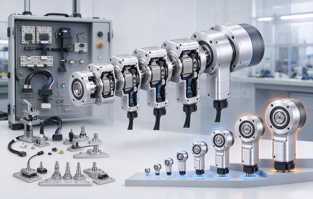
Six Functional Groups Inside the Joint Module Housing
A Laifual Drive joint module has six functional groups, each determining part of what the arm designer must solve around the axis.
The gear stage is a strain wave set of flexspline, circular spline, and wave generator, giving a high reduction ratio in a coaxial layout. Its kinematics are set out in how strain wave gears work. Its output runs on an integrated cross roller bearing that carries combined radial, axial, and moment loads, so the arm needs no separate output bearing or housing.
Actuation comes from a permanent magnet servo motor with class F insulation rated at 155 °C. An absolute encoder provides feedback and retains position and multi-turn counts after a power loss, supporting dual loop control.
Drive electronics are integrated in the 48 V DC low voltage series, removing the standalone drive cabinet from a distributed architecture. Its enclosure reaches IP67. T type joints and selected precision bearings receive black oxide treatment, a dense oxide film that raises corrosion resistance.
Where an axis needs no module, the same gear technology is supplied as a component.
Parameter Definitions and Design Criteria
Selection rests on a small set of defined quantities, each with an operating point that must be stated with the number. Rated torque is the permissible continuous load torque at a rated input speed of 2000 r/min. If an axis runs faster, the available continuous torque falls.
The average load torque Tav is the torque the reducer sees over a full duty cycle, computed from the torque and time share of each phase. It sets the frame size, which must allow at least Tav. Reduction ratio sits on the other side of the same tradeoff, and how gear ratios work sets out how ratio, input speed, and output torque move together. Ni av and Ni max are compared against the catalog range for the chosen ratio and frame.
Unit type modules carry the output bearing. They add a moment load check at the worst arm posture: maximum moment load, bearing life, and static safety factor. Positioning accuracy is quoted at plus or minus 15 arc seconds, design life at 10,000 to 15,000 hours, and backlash by series at up to 60, 30, or 20 arc seconds.
The delta tooth profile, a multi-segment variable curvature arc form derived from the double circular arc profile, raises load capacity by 15% to 30%. It lowers temperature rise by 8 to 10 °C and reduces the area affected by tooth flank fatigue pitting by more than 30%. Continuous running life extends beyond 15,000 hours.
| Parameter | Definition | Limit or value |
|---|---|---|
| Rated torque | Permissible continuous load torque | Defined at 2000 r/min input |
| Average load torque Tav | Torque averaged over a full duty cycle | At or below the permissible average load torque |
| Ni av and Ni max | Average and maximum input speed | Within the catalog range for the ratio and frame |
| Maximum moment load | Combined load on the integrated cross roller bearing | Checked for unit type modules |
| Bearing life and static safety factor | Service life of the output bearing | Checked for unit type modules |
| Positioning accuracy | Output position error | Plus or minus 15 arc seconds |
| Backlash | Lost motion at the output | Up to 60, 30, or 20 arc seconds by series |
| Design life | Rated service life of the reducer | 10,000 to 15,000 hours |
| Protection class | Enclosure rating of the module | IP67 |
| Motor insulation | Winding thermal class | Class F, 155 °C |
Technical Data: The Joint Module Size Range and the Protocol Set
At Laifual Drive, joint modules cover a continuous outside diameter range from 40 mm to 190 mm, corresponding to module sizes from Size 8 to Size 45. A design team moving from a wrist axis to a base axis therefore stays inside one interface system, protocol set, and commissioning method. The strain wave gear application matrix maps each size band to the axes it typically serves.
| Spectrum element | Specified range | Engineering note |
|---|---|---|
| Module outer diameter | 40 mm to 190 mm | Continuous, no missing size step |
| Small end | 40 mm | Approximately reducer size 8 |
| Large end | 170 mm to 190 mm | 170 mm frame, approximately reducer size 40 |
| Drive variants | 48 V DC low voltage, 220 V AC high voltage | DC models L40I to L190I, AC models M70 to M190 |
| Payload class | 3 kg to 20 kg | Light collaborative to industrial arm axes |
| Reducer sizes | Size 3 to size 58 | FSS, FSF, FSN, FSG, FHT, FHG, FHD, FHN, FBS-U, FBS-C, Mini |
| Reducer outer diameter | 13 mm to 246 mm | Overlaps the module envelope range |
| Reduction ratio | 30:1 to 160:1 | Selected per axis from torque and speed |
Communication options vary by product series. The 48 V DC low-voltage series supports CANopen, CAN FD, EtherCAT and Modbus, while the 220 V AC high-voltage series supports BiSS-C and TAMAGAWA. This range of communication options allows customers to select the interface that best fits their control architecture and application requirements.
| Protocol | Category | Engineering role in the module |
|---|---|---|
| BiSS-C | Serial encoder interface | Absolute position and multi-turn feedback |
| TAMAGAWA | Serial encoder interface | Absolute position and multi-turn feedback |
| CANopen | Fieldbus | Distributed control, -C low voltage version |
| CAN FD | Fieldbus | Same control architecture as CANopen |
| EtherCAT | Industrial Ethernet | -E low voltage version |
| Modbus | Fieldbus | Supported alongside the bus options above |
Size, protocol, and interface consistency are what make a spectrum usable rather than merely complete. The same harmonic reducer range backs the module sizes, covering size 3 through size 58 at ratios of 30:1 to 160:1, so module and component follow the same sizing logic.
Selection and Design Procedure
The procedure below places a module on one axis and is repeated for each axis of the arm.
- Build the axis table: required continuous torque, peak torque during acceleration, maximum speed, and reflected inertia of the payload and the arm segments beyond that axis.
- Compute the average load torque Tav from the duty cycle and confirm it is at or below the permissible average load torque of the candidate size. Frame size follows from Tav, not from peak torque.
- Check input speed: compare Ni av and Ni max for the cycle against the catalog range of the selected ratio and frame, with rated torque defined at 2000 r/min input.
- Check the bearing for unit type modules: maximum moment load, bearing life, and static safety factor at the worst arm posture.
- Choose the drive variant and protocol version. Distributed drives along the arm take 48 V DC low voltage, while 220 V AC high voltage suits axes that need more power and a large hollow shaft. The -C or -E version covers CANopen or EtherCAT on the low voltage side.
- Fix the accuracy class. Backlash by series at up to 60, 30, or 20 arc seconds and positioning accuracy at plus or minus 15 arc seconds must be compared against the axis requirement before the ratio is fixed.
- Confirm continuity: identify the next size up inside the same family before the drawing is released. A load increase in the prototype phase then changes the module, and not the mounting pattern or control code.
Installation, Sealing, and Commissioning Checks
Installation and maintenance follow the interface data of the module and the sealing data of the reducer. FHT-I, FHT-II, and FHT-V configurations specify oil seal and groove dimensions. Assembly requires the input fixed end sealed against the circular spline and flexspline, the output end against the circular spline, and the flexspline cavity filled with grease. Three points are worth checking on site.
- Confirm the mounting pattern and flange tolerance match the drawing before the joint is bolted into a load path.
- Keep the duty cycle inside the envelope the selection procedure established, because a joint above its thermal operating point loses life before it loses accuracy.
- Record the protocol version and encoder parameters at commissioning, since the absolute encoder keeps position and multi-turn counts across a power loss.
Where an axis needs no module, the same gear technology is applied as a component. The Mini series covers small envelopes and the hat type FHT covers hollow shaft routing.
Design Consequences of a Continuous Size Range
A continuous joint module size range moves the integration cost of a multi-axis arm out of the machine builder’s scope and into the supplier product matrix.
Protocol options vary by joint module series and configuration, providing multiple interface choices across the product range: BiSS-C, TAMAGAWA, CANopen, CAN FD, EtherCAT, and Modbus. With that in place, interface fragmentation, specification gaps, duplicated qualification, and a broken upgrade path stop driving the program schedule. Specifying the size range and its interface standard before the axis drawing is released keeps a load increase inside the same family. One size up then replaces the module rather than the mounting pattern or the control code.