
Torque Sensing Approaches in Robot Joints
Compare motor current estimation, joint torque sensors, and wrist sensors. Discover how integrated torque sensing enables precise force control and drag teaching.
 September 06, 2026
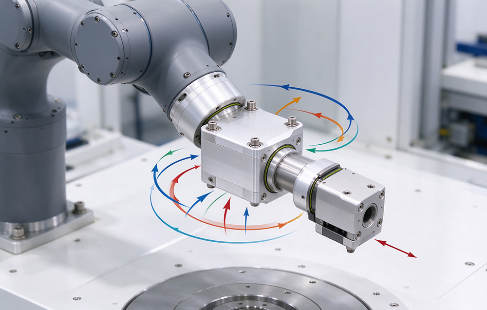
 > Torque Sensing Approaches in Robot Joints
Joint torque sensing measures the moment carried by a robot joint about its own axis. That measurement becomes an electrical signal and reaches the controller inside one control cycle, which is short enough for the control loop to act on it. Torque sensing separates a machine able to move to a position from one able to control the force it applies on the way there. Force-limited motion is otherwise inferred from position error, the quantity a stiff positioning loop is built to suppress.
Torque can be estimated from motor winding current, measured by a sensing element inside the joint, or measured outside the joint at the wrist with a multi-axis force and torque sensor. All three routes differ in the quantity they observe, in the bandwidth and accuracy they deliver, and in the design work they force into the product.
This article sets out the principle and the applicable envelope of each route, and compares them along bandwidth, accuracy, and integration cost. It then explains why force control favors measurement inside the joint drivetrain. Part of that answer lies in the rest of the joint module: an integrated drive and encoder board, and dual-loop position control.
Signal Paths from Load to Controller
Force control asks three questions. Has the joint met an unexpected obstacle, is it applying the force the process requires, and can it be moved by hand for a teaching path? Those answers sit at different points along the chain of motor, reducer, link, and tool. An estimate from motor current observes upstream of every source of friction and compliance in the drive train. A sensing element on the joint shaft observes downstream of the transmission, so the measurement includes what the external load does to the structure. A wrist sensor observes at the far end of the arm and returns the resultant at the tool, not the contribution of a single axis.
Torque Estimation from Motor Current
Servo motor output torque is approximately proportional to its winding current. A drive that already regulates current therefore already holds a torque signal, with no additional hardware, no mechanical change, and no cost per axis. That proportionality is the weak point. This ratio shifts with winding temperature, magnetic saturation, friction, and transmission efficiency, and the friction and hysteresis of a strain wave gear vary with load, speed, and lubrication state. Estimates obtained this way typically carry an error of a few percent to more than ten percent of transmitted torque.
On an axis carrying a large gravity load, a few percent of a large torque can exceed the contact force the process is meant to regulate. Such an estimate then cannot separate the quantity of interest from the quantity that dominates it. Such a route therefore suits coarse force control, such as detecting a collision or a jam and stopping the axis. It suits contact force regulation less well, because there the commanded force is small relative to the load already carried. That limit belongs to the observation point, and no filtering removes it.
Strain-Based Sensing Inside the Joint
A second route places the sensing element inside the joint and measures the torque carried by the joint shaft directly. The common implementation bonds strain gauges to a structural member in the load path, such as the output flange or a dedicated elastic element. Bridge output maps to torque once the element has been calibrated.
The structure that carries the load produces the signal, so the reading follows changes in external force. Motor effort does not enter it. Bandwidth is set by the compliance and mass of the instrumented element and by its acquisition electronics, not by the dynamics of the reducer.
Its cost is paid in design, not in hardware. Space for the element, the load path through it, and its cabling route have to be reserved while the joint structure is defined. Each unit has to be calibrated individually and compensated for temperature drift, or the reading moves with duty conditions. A force-controlled joint module is therefore designed from the structure outward, not by attaching a sensor to a standard joint.
Six-Axis Force and Torque Sensing at the Wrist
The third route mounts a six-axis force and torque sensor at the end of the arm. It reports the three force and three moment components acting on the tool, which is the quantity a process such as grinding or assembly needs. This route is the most established of the three in production use.
Its limitation is resolution. The sensor measures the resultant applied to the wrist, and no arithmetic recovers the contribution of an individual joint from it. Joint-level quantities such as the torque each reducer carries therefore remain unknown to the control system. That sensor also sits outside the wrist, adding volume, mass, and cabling where added mass costs the most in dynamic response. Cost per unit is high enough that instruments cannot be distributed across every joint of a multi-axis machine.
Comparing the Three Routes Along Three Dimensions
| Dimension | Estimation from Motor Current | Sensing Inside the Joint | Sensor at the Wrist |
|---|---|---|---|
| Quantity observed | Winding current, upstream of the transmission | Torque on the joint shaft, downstream of the reducer | Resultant force and moment at the tool |
| Accuracy | A few percent to more than ten percent of transmitted torque | Set by element calibration and temperature compensation | High at the tool, but a single resultant only |
| Bandwidth | Set by the current loop and the position cascade | Set by the instrumented element and its acquisition electronics | Set by the sensor and its conditioning electronics |
| Reducer friction and hysteresis | Included in the estimate and not separable from load torque | Excluded, because the measurement is taken downstream of the reducer | Excluded |
| Design impact | None | Space, load path, and cable routing reserved at design stage | Wrist interface plus added volume, mass, and cabling |
| Cost per axis | None | Calibration and compensation for each unit | One instrument per arm, not distributed across the joints |
| Where it fits | Coarse force control, collision, and jam detection | Distributed force sensing, drag teaching, joint-level force control | Process-level force control in grinding and assembly |
This pattern is structural, not incremental. Moving the observation point downstream of the transmission removes reducer friction and hysteresis in one step. That requirement then moves into the mechanical design of the joint itself.
Combining the Routes Rather Than Choosing Between Them
All three are complementary, and the usual arrangement runs joint-level and wrist-level sensing together. At the joint level, the signal supplies the torque of each axis and supports distributed force sensing, collision detection, and safety judgment. At the wrist, it supplies a high-accuracy resultant for the process itself. Its controller then closes the force loop using both.
The closer the observation point is to the source of the torque, the cleaner the signal, and the closer it is to the tool, the higher the accuracy of the process quantity. A design that carries both covers the joints with distributed information and the tool with a calibrated resultant.
Engineering Prerequisites for Joint-Level Torque Sensing
| Prerequisite | What It Demands | What Is Lost If It Is Deferred |
|---|---|---|
| Structural reservation | Space for the sensing element, a defined load path through it, and a route for its cabling | Accuracy and reliability, because a retrofit cannot recreate a clean load path |
| Calibration and compensation | Calibration of the sensing output for each unit and compensation for temperature drift | Accuracy that holds only in the conditions in which the unit was set up |
| Real-time link | Sampling, transmission, and closed-loop execution inside one short enough cycle | Loop performance, which is why millisecond-class communication is a standard requirement in force-controlled products |
Communication protocols depend on the voltage series. The 48 V DC low-voltage joint modules support CANopen, CAN FD, EtherCAT, and Modbus. The 220 V AC high-voltage joint modules support BiSS-C and TAMAGAWA. The protocol and feedback configuration should be confirmed for the selected model.
Integration Inside the Joint Module
Torque sensing capability tracks how much of the drive train is already integrated. Where the motor, harmonic reducer, encoder, servo drive, and sensing element share one housing, sampling and execution sit on a short electrical path inside a single enclosure. Added delay and electrical interference are then easier to hold down. One alternative is a sensor signal that leaves the joint, passes through a cabinet, and returns as a command.
Dual-Loop Position Control and Absolute Feedback
Dual-loop position control belongs to the same argument. The output side of the reduction enters the loop alongside the motor side, so the controller observes the load end of the reducer instead of inferring it through the gear. That general layered arrangement is described in what a servo actuator is. An absolute encoder that retains position and multi-turn count through a power loss completes the picture. That comparison between an integrated unit and separate components is set out in the actuator robot basics background.
Distributed Force Sensing in the Low-Voltage Family
This low-voltage family carries the drive, the encoder interface, and the torque signal in one package. That makes distributed force sensing practical on an arm with many axes. Range and detail are on the DC low voltage joint modules page.
Force-controlled modules of this class appear most often in collaborative and humanoid work, where a hand-guided move and a safe collision response matter as much as positional accuracy. A survey of robot actuators in humanoid designs describes that duty, and the wider set of duties is covered under robotics applications. One interface, one calibration route, and one set of bus options run from 40 mm to 190 mm outside diameter. An arm can be specified along its whole length from the joint modules family.
Module Data for a Force-Controlled Axis
| Item | Published Coverage |
|---|---|
| Joint torque sensing | Integrated in the force-controlled joint modules with real-time torque feedback for drag teaching, collision detection, and torque control |
| Joint module outside diameter | 40 mm to 190 mm, continuous across the range |
| Supply forms | 48 V DC with built-in servo drive; 220 V AC with large hollow shaft support |
| Models | DC 48 V: L40I, L52I, L60I, L70I, L80I, L90I, L110I, L142I, L170I, L190I; AC 220 V: M70, M80, M90, M110, M142, M170, M190 |
| Communication protocols | DC 48 V: CANopen, CAN FD, EtherCAT, and Modbus; AC 220 V: BiSS-C and TAMAGAWA |
| Feedback behavior | Absolute encoder retaining position and multi-turn count through power loss; dual-loop position control |
| Positioning accuracy | ±15 arcseconds |
| Design life | 10,000 to 15,000 hours |
| Protection and insulation | IP67 enclosure; class F motor insulation at 155 °C |
| Payload and range of use | 3 kg to 20 kg, from collaborative robots and humanoid robots to precision assembly |
Choosing a Torque Sensing Approach
Selection follows the quantity the control loop has to resolve. A machine that needs only a threshold on joint torque for collision detection can be served by current estimation, which costs no hardware and no design time. A machine that must regulate contact force at each axis, or move an axis by hand for teaching, needs the observation point inside the joint. Space for the element, per-unit calibration, temperature compensation, and a short real-time link then belong in the design budget from the start. Where the process is defined by the resultant at the tool, a wrist sensor stays necessary alongside the joint-level signal.
Fixing the Observation Point at Design Stage
One practical rule is to fix the observation point for each control loop while the structure is still on the drawing. Joint-level sensing placed at that stage costs space, calibration, and a communication cycle. That same capability added after the mechanism is built costs accuracy that cannot be recovered. Those three were already settled by other decisions.
Explore Integrated Force Feedback Solutions
Speak with our robotics actuator engineers for integrated torque sensor calibration data, dual-loop encoder pinouts, and custom humanoid joint module designs.